Last year, we started our vision journey by auto-aiming just with the horizontal angle from our Limelight. However, we quickly realized the utility of calculating the robot’s position based on a vision target instead. By integrating that data with regular wheel odometry, we could auto-aim before the target was in sight, calculate the distance for the shot, and ensure our auto routines ended up at the correct locations (regardless of where the robot was placed on the field).

Our main objective over the past week was to create a similar system for the 2022 vision target around the hub. This meant both calculating the position of the robot relative to the target and smoothly integrating that position information with regular odometry.

While both the Limelight and PhotonVision now support target grouping, we wanted to fully utilize the data available to us by tracking each piece of tape around the ring individually (more on the benefits of that later). Currently, only PhotonVision supports tracking multiple targets simultaneously; for our testing, we installed PhotonVision on the Limelight for our 2020 robot.

The Pipeline

This video shows our full vision/odometry pipeline in action. Each step is explained in detail below.

1. PhotonVision runs the HSV thresholding and finds contours for each piece of tape. Using the same camera mount as last year, we found that the target remains visible from ~4ft in front of the ring to the back of the field (we’ll adjust the exact mount for the competition robot of course). In most of that range, 4 pieces of tape are visible. We’ve never seen >5 tracked consistently, and less optimal spots will produce just 2-3. Currently, PhotonVision is running at 960×720; the pieces of tape can be very small on the edges, so every pixel helps. The robot code reads the corners of each contour, which are seen on the left of the video.
2. Using the coordinates in the image along with the camera angle and target heights, the code calculates a top-down translation from the camera to each corner. This requires separating the top and bottom corners and calculating each set with the appropriate heights. These translations are plotted in the middle section of the video.
3. Based on the known radius of the vision target, the code fits a circle to the calculated points. This is where we see the key benefit of plotting 12+ points rather than just 2 (as we did last year). When the robot is stationary, the position of the circle stays within a range of just 0.2-0.5 inches frame-to-frame. Last year, we could easily see a range of >3 inches. While the translations to each individual corner are still noisy, the circle fit is able to average all of that out and stay in almost exactly the same location. It’s also able to continue solving even when just two pieces of tape are visible on the side of the frame; so long as the corners fall somewhere along the circumference of the vision ring, the circle fit will be reasonably accurate.
4. Using the camera-to-target translation, the current gyro rotation, and the offset from the center of the robot to the camera, the code calculates the full robot pose. This “pure vision” pose is visible as a translucent robot to the right of the video. Based on measurements of the real robot, this pose is usually within ~2 inches of the correct position. For our purposes, this is more than enough precision.
5. Finally, the vision pose needs to be combined with regular wheel odometry. We started by utilizing the DifferentialDrivePoseEstimator class, which makes use of a Kalman filter. However, we found that adding a vision measurement usually took ~10ms, which was impractical during a 20ms loop cycle. Instead, we put together a simpler system; each frame, the current pose and vision pose are combined with a weighted average (~4% vision). This means that after one second of vision data, the pose is composed of 85% vision. It also uses the current angular velocity to adjust this gain — the data tends to be less reliable when the robot is moving. This system smoothly brings the current pose closer to the vision pose, making it practical for use with motion profiling. The final combined pose is shown as the solid robot to the right of the video.

Where applicable, these steps also handle latency compensation. New frames are detected using an NT listener, then timestamped (using the arrival time, latency provided by PhotonVision, and a constant offset to account for network delay). This timestamp is used to retrieve the correct gyro angle and run the averaging filter. Note that the visualizations shown here don’t take this latency into account, so the vision data appears to lag behind the final pose.

More Visualizations

This video shows the real robot location next to the calculated vision pose. The pose shown on the laptop is based on the camera and the gyro, but ignores the wheel encoders. This video was recorded with an older version of the vision algorithm, so the final result is extra noisy.

This was a test of using vision data during a motion profile – it stops quickly to intentionally offset the odometry. The first run was performed with the vision LEDs lit, meaning the robot can correct its pose and return to the starting location. The second run was performed with the LEDs off, meaning the robot couldn’t correct its pose and so it returned to the incorrect location.

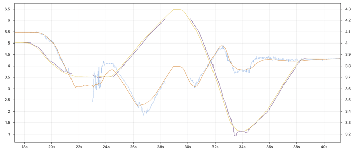
This graph shows the x and y positions from pure vision along with the final integrated pose.

• Vision X = purple
• Vision Y = blue
• Final X = yellow
• Final Y = orange

The final pose moves smoothly but stays in sync with the vision pose. The averaging algorithm is also able to reject noisy data when the robot moves quickly (e.g. 26-28s).

Logging

This project has been a perfect opportunity to use our new logging framework.

For example, at one point during the week, I found that the code was only using one corner of each piece of tape and solving it four times (twice using the height of the bottom of the tape and twice using the top). I had grabbed a log file to record a video while I was running on code without uncommitted changes. On a whim, I switched to the original commit and replayed the code in a simulator with some breakpoints during the vision calculation. I noticed that the calculated translations looked odd, and was able to track down the issue. After fixing it locally, I could replay the same log and see that the new odometry positions were shifted by a few inches throughout the test.

Logging was also a useful resource when putting together the pipeline visualization in this post. We had a log file from a previous test, but it was a) based on an older version of the algorithm and b) didn’t log all of the necessary data (like the individual corner translations). However, we could replay the log with up-to-date code and record all of the extra data we needed. Advantage Scope then converted the data to a CSV file that Python could read and use to generate the video.

Code Links

• NT listener to read PhotonVision data (here)
• Calculation of camera-to-target translation (here)
• Circle fitting class (here)
• Method to combine vision and wheel odometry (here)

As always, we’re happy to answer any questions.